Example Side-Channel Acquisition

In this notebook we show how to do an acquisition using the secbench framework, more precisely, the secbench.api and secbench.storage modules.

Bench and Hardware Setup

import logging

import matplotlib.pyplot as plt
import numpy as np

from secbench.api import get_bench
from secbench.api.simulation import SimulatedScope
from secbench.storage import Dataset, Store

First, we enable the logging and create a Bench.

logging.basicConfig(level=logging.INFO)

bench = get_bench()

INFO:secbench.api.bench:SECBENCH_USER_CONFIG not defined, no user configuration loaded

INFO:secbench.api.bench:SECBENCH_SCOPENET not defined, skipping registration of VxiScanner

INFO:secbench.api.bench:SECBENCH_PYVISA_BACKEND not defined, skipping registration of PyVisaScanner

We now grab a scope.

Note

To make the notebook executable without real hardware, we create a simulated scope and register it manually.

scope = SimulatedScope(channel_names=["1", "2"])
bench.register(scope)

In a real experiment, the previous cell is not needed, you only need to do:

scope = bench.get_scope()

Here we define the parameters of the acquisition:

total_size = 300  # How many traces to acquire.
batch_size = 100   # Size of batches acquisired for segmented acquisition.
n_batches = total_size // batch_size

Then, we need to define some device under test (DUT). It is specific to each experiment. The goal of the device under test is to perform some computation (AES, RSA, ECC or other) and ideally generate a trigger signal.

For this example, we suppose that the DUT processes a 16 byte plaintext. Our implementation below will force a trigger on the scope. In a real side-channel experiment, you will probably need to open a serial port, send the plaintext to the target, etc.

class Dut:
    def process(self, plaintext):
        scope.force_trigger()

Now, we instanciate a DUT:

dut = Dut()

We generate some inputs for the acquisitions. Remember that the DUT processes 16-bytes plaintexts in our example.

pts = np.random.randint(0, 256, size=(total_size, 16), dtype=np.uint8)

Dataset Initialization

Now, we can create a Store and a Dataset inside it for our acquisition. If we were to do multiple acquisitions, we could create multiple Dataset with different names.

store = Store('example_campaign.hdf5', mode='w')

ds = store.create_dataset('my_acquisition', total_size, 'data', 'pts')

Acquisition

To do an acquisition, we should first setup the scope and configure the trigger. This can be done manually or via the Scope API. We have a whole tutorial dedicated on this topic in Using Scopes.

Here is an example configuration. Do not forget to update it if you do a real experiment.

scope["1"].setup(range=3, offset=0)
scope["2"].setup(range=10e-3, offset=0)
scope.set_horizontal(samples=200, interval=1e-8)
scope.set_trigger(channel="1", level=1.2)

A good practice is to dump the scope configuration and save it in the dataset.

This is how you get the scope configuration (we only query channels we use in our acquisition):

scope_config = scope.config(channels=["1", "2"])
scope_config

{'scope_name': 'SimulatedScope',
 'scope_description': 'simulated scope',
 'scope_horizontal_samples': 200,
 'scope_horizontal_interval': 1e-08,
 'scope_horizontal_duration': 2e-06,
 'scope_channel_1': {'coupling': <Coupling.dc: 'dc'>,
  'offset': 0,
  'range': 3,
  'decimation': <Decimation.sample: 'sample'>,
  'enabled': True},
 'scope_channel_2': {'coupling': <Coupling.dc: 'dc'>,
  'offset': 0,
  'range': 0.01,
  'decimation': <Decimation.sample: 'sample'>,
  'enabled': True}}

This is how you save the scope configuration in a dataset. By convention, we call the asset “scope_config.json”.

ds.add_json_asset("scope_config.json", scope_config)

If your scope supports it, segmented acquisitions can drastically speed-up the acquisition process.

scope.segmented_acquisition(batch_size)

Now let’s get some traces! Here is a generic acquisition loop:

for batch_number in range(n_batches):
    # We retrieve 10 batches of 100 traces each
    start, end = batch_number * batch_size, (batch_number + 1) * batch_size
    scope.arm()
    for exec_number in range(start, end):
        dut.process(pts[exec_number])
    scope.wait()
    # Query traces from the scope.
    traces, = scope.get_data("1")
    # Add the batch of traces and pts to the dataset.
    ds.extend(traces, pts[start:end])

del ds
store.close()
del store

Reloading the Dataset

This section shows how to reload the dataset. First, it is a good idea to inspect the data using the secbench-db status command. We can see for the “my_acquisition” dataset, we have size=300, which means the dataset was fully populated.

!secbench-db status example_campaign.hdf5

ROOT
 +-- my_acquisition
     +-- capacity: 300
     +-- size: 300
     +-- fields
     |   +-- data: shape=(300, 200), dtype=int8
     |   +-- pts: shape=(300, 16), dtype=uint8
     +-- assets
         +-- scope_config.json: shape=(390,), dtype=uint8

Now, we open the store in read-only mode. For analysis, we have no reason to open the store in write mode.

store_reload = Store("example_campaign.hdf5", mode="r")

ds = store_reload["my_acquisition"]

ds_data = ds["data"]
ds_pts = ds["pts"]

When you reload data, as shown in the previous cell, the data returned are not numpy arrays. At this point the data are not loaded in RAM, which is a good thing when you have huge datasets.

print(type(ds_data))

<class 'h5py._hl.dataset.Dataset'>

Luckily, the ds_data and ds_pts support almost all numpy array methods.

print(ds_data.dtype)
print(ds_data.shape)

int8
(300, 200)

ds_data_dram = ds_data[:]
ds_pts_dram = ds_pts[:]

print(type(ds_data_dram))

<class 'numpy.ndarray'>

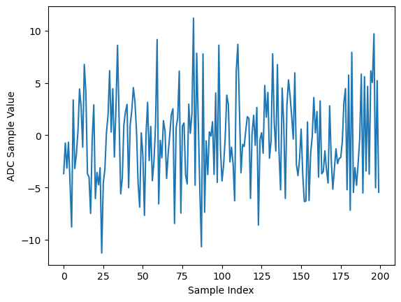
At this point, you can do all side-channel processing you want. Our simulated data are not very interesting, but we can plot the mean trace for example:

plt.plot(np.mean(ds_data, axis=0))
plt.xlabel("Sample Index")
plt.ylabel("ADC Sample Value")
plt.show()

You can also recover the configuration from the scope:

ds_scope_config = ds.get_json_asset("scope_config.json")

ds_scope_config

{'scope_name': 'SimulatedScope',
 'scope_description': 'simulated scope',
 'scope_horizontal_samples': 200,
 'scope_horizontal_interval': 1e-08,
 'scope_horizontal_duration': 2e-06,
 'scope_channel_1': {'coupling': 'dc',
  'offset': 0,
  'range': 3,
  'decimation': 'sample',
  'enabled': True},
 'scope_channel_2': {'coupling': 'dc',
  'offset': 0,
  'range': 0.01,
  'decimation': 'sample',
  'enabled': True}}

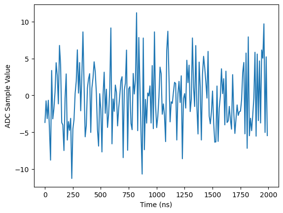
One nice thing is that we can recompute the real time scale of traces.

time_ns = 1e9 * scope_config["scope_horizontal_interval"] * np.arange(ds_data.shape[1])

plt.plot(time_ns, np.mean(ds_data, axis=0))
plt.xlabel("Time (ns)")
plt.ylabel("ADC Sample Value")
plt.show()